PRX Part 3 — Training a Text-to-Image Model in 24h!


Introduction
Welcome back 👋
In the last two posts (Part 1 and Part 2), we explored a wide range of architectural and training tricks for diffusion models. We tried to evaluate each idea in isolation, measuring throughput, convergence speed, and final image quality, and tried to understand what actually moves the needle.
In this post, we want to answer a much more practical question:
What happens when we combine all the tricks that worked?
Instead of optimizing one dimension at a time, we’ll stack the most promising ingredients together and see how far we can push performance under a strict compute budget.
To make things concrete, we’re doing a 24-hour speedrun:
- 32 H200
- ~$1500 total compute budget (2$/hour/GPU)
This is very far from the early diffusion days, where training competitive models could cost millions of dollars. The goal here is to demonstrate how much the field has evolved and how far careful engineering can take you in just a single day of training.
This speedrun is not just a fun experiment. It will likely serve as the foundation for our large-scale training recipe going forward.
Alongside the results, we’re also open-sourcing our code (Github link), which contains:
- The training code used for this speedrun
- The experimental framework from the previous blog post
So you can reproduce, modify, and extend everything yourself.
The Training Recipe
Now let’s walk through what went into this 24h run.
X-prediction and Training in the Pixel Space
We use the x-prediction formulation from Back to Basics: Let Denoising Generative Models Denoise [Li and He, 2025]. As seen in Part 2, this enables training directly in pixel space and eliminates the need for a VAE altogether. We use a patch size of 32 and use a 256-dimensional bottleneck in the initial token projection layer. This design keeps the sequence length under control, making pixel-space training computationally manageable even at higher resolutions.
At 512px, the sequence length is:
At 1024px, the sequence length becomes:
Instead of following the usual 256px → 512px → 1024px schedule, we start directly at 512px and then fine-tune at 1024px.
With controlled token counts and modern hardware, pixel-space training is no longer prohibitive. It is simply a cleaner and more direct formulation.
Perceptual Losses
One very nice side effect of predicting directly in pixel space is that we can reuse a whole toolbox from classical computer vision.
When your model outputs latents, perceptual supervision becomes awkward. You either have to decode back to pixels or define losses in a learned latent space that may or may not align with human perception. Once you predict pixels directly, everything becomes straightforward again. You can plug in perceptual losses exactly as they were originally designed.
We take inspiration from the paper PixelGen: Pixel Diffusion Beats Latent Diffusion with Perceptual Loss [Ma et al.], where the authors introduce additional perceptual objectives on top of the diffusion loss. They show that adding perceptual signals can noticeably improve convergence speed and final visual quality.
For this 24h run, we add two auxiliary losses:
- LPIPS ([Zhang et al.])
- A DINO-based perceptual loss (we use DINOv2 [Oquab et al.])
The idea is simple: In addition to the standard flow matching objective, we encourage the predicted clean image to match the target image in a perceptual feature space. LPIPS captures low-level perceptual similarity, while DINO features provide a stronger semantic signal.
We keep the same overall idea as the paper, but we tweaked a few details. In our experiments, we empirically found that it worked better to:
- apply the perceptual losses on pooled full images instead of patch-wise features
- apply them at all noise levels
These are small implementation details, but in our setting they consistently gave better results.
We used a weight of 0.1 for the LPIPS loss and 0.01 for the DINO perceptual loss, matching the values recommended in the original paper.
These losses are lightweight compared to the main transformer forward pass, and in our setup they add only a small overhead while providing a consistent quality boost.
Token Routing with TREAD
To make each step cheaper, we use token routing with TREAD [Krause et al., 2025]), which randomly selects a fraction of tokens and lets them bypass a contiguous chunk of transformer blocks, then re-injects them later so nothing is dropped.
We picked TREAD over SPRINT (Park et al., 2025) mostly for simplicity, and because the extra complexity of SPRINT did not feel worth the fairly small additional compute savings in our setting (sequence length 64 vs. 128 with TREAD at 512px).
Following the TREAD recipe, we route 50% of the tokens from the 2nd block to the penultimate block of the transformer.
Routed models can look worse under vanilla CFG, especially when undertrained, so we implemented a simple self-guidance scheme inspired by Guiding Token-Sparse Diffusion Models (Krause et al., 2025), which guides using a dense vs. routed conditional prediction instead of relying on an unconditional branch.
Representation Alignment with REPA and DINOv3
We used REPA [Yu et al., 2024] for representation alignment.
For the teacher, we went with DINOv3 [Siméoni et al. 2025] since it gave the best quality improvements in our previous experiments.
Concretely, we apply the alignment loss once,at the 8th transformer block with a loss weight of 0.5.
Since we combine REPA with TREAD routing, we only compute the alignment loss on the non-routed tokens, meaning the tokens that actually go through the blocks where we apply the loss. This keeps the REPA signal consistent and avoids comparing features for tokens that skipped the computation path.
Optimizer: Muon
We used the Muon optimizer, using the FSDP implementation from muon_fsdp_2, since it showed a clear improvement over Adam in our previous runs.
Muon is only applied to 2D parameters (basically matrices). Everything else (biases, norms, embeddings, etc.) is optimized with Adam, which is why the config has two parameter groups.
| Group | What it applies to | Key params we used |
|---|---|---|
| Muon | 2D parameters | lr=1e-4, momentum=0.95, nesterov=true, ns_steps=5 |
| Adam | all non-2D parameters | lr=1e-4, betas=(0.9, 0.95), eps=1e-8 |
Training Settings
We trained on three publicly available synthetic datasets:
- Flux generated (1.7M), lehduong/flux_generated
- FLUX-Reason-6M (6M), LucasFang/FLUX-Reason-6M
- midjourney-v6-llava (1M), brivangl/midjourney-v6-llava which we re-captioned with Gemini 1.5 to make prompts more consistent and cut down caption noise.
The schedule is basically: go fast at 512, then sharpen at 1024:
- 512px for 100k steps with batch size 1024
- 1024px for 20k steps with batch size 512 without REPA.
We also keep an EMA of the weights for sampling and eval:
smoothing = 0.999update_interval = 10baema_start = 0ba
Results and Closing Thoughts
Below are the evaluation curves we tracked throughout the run and a few sample grids from the final checkpoint:


For a one day training run, this is already a pretty solid place to be. The model is not flawless yet (you can still spot some texture glitches, occasional weird anatomy, and it can get a bit shaky on very hard prompts), but it is clearly usable. Prompt following is strong, the overall aesthetic is consistent, and the 1024 stage mostly does what we want: sharpen details without breaking composition.
The key takeaway is that we're very close. The remaining issues look more like undertraining artifacts and limited data diversity than signs of a structural flaw in the recipe. The failure modes are consistent with what you’d expect from a model that simply hasn’t seen enough varied data yet. With more compute and broader coverage, this exact setup should continue improving in a fairly predictable way.
Zooming out, this speed run also highlights how far diffusion training has come. By combining pixel-space training, efficient routing, representation alignment, and lightweight perceptual guidance, you can now get a meaningful model in about a day on a budget that would have sounded unrealistic not that long ago.
What’s next?
This 24h run is just a starting point, not the finish line. Next, we will keep pushing the same recipe with a bit more scale and iterate on the dataset mix and captioning.
All the code and configs behind this speedrun, as well as the full experimental framework used throughout Part 1 and Part 2, are available in the PRX repository: https://github.com/Photoroom/PRX.
While we don’t redistribute the exact training datasets used in this run, the pipeline is fully configurable and designed to be easily adapted to your own data. You can plug in different datasets, tweak individual components (TREAD, REPA, perceptual losses, Muon, etc.), and run controlled experiments with minimal friction. Our goal is to make this a practical playground for fast diffusion research, and we hope the community will use it to explore, benchmark, and iterate on these techniques in their own setups.
If you made it this far, thank you for reading. We would also love to have you join our Discord community, where we share PRX progress and results, and discuss anything diffusion and text-to-image related.
Goodbye for now, and stay tuned for the next round of experiments! 🚀
Acknowledgements.
This speedrun was inspired by several recent efforts exploring fast and low-cost training of diffusion models. If you're interested in speedrunning text-to-image models, we encourage you to check out the following works:
- Haridas, A., Shen, T., Yu, J. Nitro-T: Training a Text-to-Image Diffusion Model from Scratch in 1 Day. https://rocm.blogs.amd.com/artificial-intelligence/nitro-t-diffusion/README.html
- Bhanded, S. Speedrunning ImageNet Diffusion. https://arxiv.org/abs/2512.12386
- Sehwag, V., Kong, X., Li, J., Spranger, M., Lyu, L. Stretching Each Dollar: Diffusion Training from Scratch on a Micro-Budget. https://arxiv.org/abs/2407.15811
- Yeh, S.-Y. Home-made Diffusion Model from Scratch to Hatch. https://arxiv.org/abs/2509.06068